K-nearest neighbors

K-nearest neighbors is a simple form of machine-learning. It is an algorithm designed to extrapolate and generalize from a given dataset. This post will cover implementing the algorithm in python with the final goal of applying it to the cifar-10 dataset.

The idea of k-nearest neighbors is to be able to make predictions of a parameter on an unseen datapoint by weighing in said parameter values of the k “closest” datapoints. It is a quite general algorithm that can be applied on top of many other machine-learning algorithms as the performance largely depends on the distance metric used.

Cifar-10

The cifar-10 dataset consists of 60000 labeled 32x32 RBG pixel images. It can be downloaded from here. Once downloaded, pickle can be used to load the batch files into a dictionary in python.

Alternatively, using keras:

from keras.datasets import cifar10

import numpy as np

X_train shape:
(50000, 3072)
Y_train shape:
(50000,)
X_test shape:
(10000, 3072)
Y_test shape:
(10000,)

categories:
['airplane', 'automobile', 'bird', 'cat', 'deer', 'dog', 'frog', 'horse', 'ship', 'truck']

The data is loaded as a vector of length $N_{batch} \cdot 3 \cdot 32 \cdot 32 = 30720000$ per batch. After concatenating, the full data vector needs to be reshaped into a matrix $X$ of dimension $N \times D = N \times 3072 = N \times 3 \cdot 32 \cdot 32$ (where $N$ is the number of samples and $D$ is the data dimension size), by using .reshape(-1, 3 * 32 * 32). Then, for example, X[0] returns the first image as a vector of length $3 \cdot 32 \cdot 32$.

Pyplot’s imshow can be used to display an image. For this, the data vector $x$ needs to be resized to $3 \times 32 \times 32$. Also since pyplot’s convention is to have the RGB information in the last axis, the RGB channel (2nd axis) has to be moved to the back using .transpose(1,2,0).

def show(x, title):

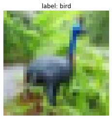
Et Voila! An ostrich.

The next step splits a dataset (X, Y) into a training and a test set, given a ratio. This is not strictly necessary, as our dataset has already been split for us. Although we can use this to work with a smaller subset for development.

def split_dataset(X, Y, ratio):

K-nearest neighbor distances

Central to the performance of the algorithm is the distance function $d(x,y)$ which measures closeness of two datapoints. Since we are working with a batch of datapoints for which we would like to make predictions, we will be working with a matrix $Dist = \{d\}_{i,j} = ||x^i - y^j||^2$ containing all the pairwise distances between each image of the training and in this case, the testing set. These pairwise distances will then be used to predict labels for all images of the testing set. A simple distance metric is the $l2$-metric, the sum of the squared distance of each pixel value.

Mathsy explanation

In the following short part, the training set and the test set will be denoted as

$X = \begin{bmatrix}- x^1 -\\ \vdots \\ - x^{N_X} -\end{bmatrix} \in N_X \times D$ and $Y = \begin{bmatrix}- y^1 -\\ \vdots \\ - y^{N_Y} -\end{bmatrix} \in N_Y \times D$ respectively.

The matrix’ entries $d_{i,j} = dist(i, j)^2 = ||x^i - y^j||^2$ contain the squared distance between the i-th image of set $X$ and the j-th image of set $Y$. An easy way for calculating this is by observing that

$||x - y||^2 = (x - y) \cdot (x - y) = x \cdot x - 2x \cdot y + y \cdot y = ||x||^2 -2x \cdot y + ||y||^2$

(where $\cdot$ denotes the dot/scalar product of vectors)

and

$X Y^\top = \begin{bmatrix}- x^1 -\\ \vdots \\ - x^{N_X} -\end{bmatrix} \begin{bmatrix}| & & | \\ y^1 & \ldots & y^{N_Y} \\| & & | \end{bmatrix} = \begin{bmatrix} x^1 \cdot y^1 & \ldots & x^1 \cdot y^{N_Y} \\ \vdots & \ddots & \vdots \\ x^{N_X} \cdot y^1 & \ldots & x^{N_X} \cdot y^{N_Y} \end{bmatrix}$

Now, starting off with the matrix $-2XY^\top$ and adding to it’s columns the vector $\begin{pmatrix}||x^1||^2\\ \vdots \\ ||x^{N_X}||^2\end{pmatrix}$
and to it’s rows the vector $\begin{pmatrix}||y^1||^2 & \ldots & ||y^{N_Y}||^2\end{pmatrix}$

results in

$\begin{bmatrix} ||x^1||^2 - 2 x^1\cdot y^1 + ||y^1||^2& \ldots & ||x^1||^2 - 2 x^1 \cdot y^{N_Y} + ||y^{N_Y}||^2 \\ \vdots & \ddots & \vdots \\ ||x^{N_X}||^2 - 2 x^{N_X} \cdot y^1 + ||y^1||^2 & \ldots & ||x^{N_X}||^2 - 2 x^{N_X} \cdot y^{N_Y} + ||y^{N_Y}||^2 \end{bmatrix} = \begin{bmatrix} d_{11} & \ldots & d_{1N_Y} \\ \vdots & \ddots & \vdots \\ d_{N_X1} & \ldots & d_{N_XN_Y} \\ \end{bmatrix}$

Thankfully, this is easily done via numpy’s broadcasting. Numpy will automatically add row/column vectors to the rows/columns of a matrix, if the dimensions match up.

def knn_distances(X, Y):

# sanity check

697.50433
697.50433

Predicting

Given an image with an unknown label, we could simply calculate its distance to all samples with known labels and then assign the label of the ‘closest’ image. This is called 1-nearest neighbor.
In the case of 1-nearest neighbor, it is quite simple. After having calculated the pairwise distances for a given set of unlabeled data, looking at the smallest value in each of the matrix’ columns corresponds, by definition, to the image of the labeled dataset ‘closest’ to each image.

def predict_1nn(dist, Y_train):

Taking into account the k closest samples, leads to K-nearest neighbors. For this, first, for each image we need to run vertically down the distance matrix and note the indices of the k-smallest numbers. Then we look at the k corresponding labels, count them and and pick the label which occurs the most.
To get the k-smallest indices of each column, we run np.argpartition() over the columns, which sorts our indices by the smallest values (it only sorts the first k-smallest, as indicated by the functions second argument).
Then we iterate through the columns to count the occurences of each label using np.bincount() and finally, we return the bin (in this case also the label) with the highest count, by applying np.argmax().

An example walking through argpartition and bincount

Code:

np.random.seed(1)

distance matrix:
[[5 8 9 5 0 0 1 7 6 9]
 [2 4 5 2 4 2 4 7 7 9]
 [1 7 0 6 9 9 7 6 9 1]
 [0 1 8 8 3 9 8 7 3 6]
 [5 1 9 3 4 8 1 4 0 3]
 [9 2 0 4 9 2 7 7 9 8]]
3-smallest indices: 
[[3 3 2 4 0 0 4 4 4 3]
 [2 4 5 5 3 5 0 2 3 2]
 [1 5 1 1 1 1 1 0 0 4]]
corresponding image's label: 
[[4 4 9 1 6 6 1 1 1 4]
 [9 1 1 1 4 1 6 9 4 9]
 [9 1 9 9 9 9 9 6 6 1]]

categories:
[0 1 2 3 4 5 6 7 8 9]

bincount of [4 9 9]:
[0 0 0 0 1 0 0 0 0 2]
label -> 9
bincount of [4 1 1]:
[0 2 0 0 1 0 0 0 0 0]
label -> 1
bincount of [9 1 9]:
[0 1 0 0 0 0 0 0 0 2]
label -> 9
bincount of [1 1 9]:
[0 2 0 0 0 0 0 0 0 1]
label -> 1
...

def knn_predict(k, dist, Y_train):

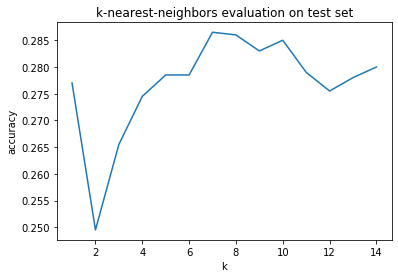
Great! We can reach an accuracy of almost 30% of our predictions on the test set with a k value of around 7. Although, you’ve probably heard of overfitting before. Our variable k is a hyperparameter which controls the behavior of our model and we are currently tuning it to best fit the test set. This means that hypothetically if we had a bunch of other hyperparameters we could all tune at once, we might be able to reach a very high accuracy by some numerical happenstance. This is why it is common practice to not look at your test set until all tuning of hyperparameters is finished and to only use it as a final evaluation.

Cross validation

One way to find which hyperparameters work best for our model is by using cross validation, a technique where you shuffle, then split your training set into multiple folds, iterating through them by using one fold as a validation set and the rest as your new temporary training set. Like this we can evaluate our model many times, only using our training set and make sure we don’t accidentally overfit.
For this, we need to write a function that returns the indices of the new training and validation set.

def cross_fold_idx(N, folds):

example

N = 11

[0 1 2 3 4 5 6 7 8 9 10]
0-th validation set yield: [0,3)
1-th validation set yield: [3,6)
2-th validation set yield: [6,9)

Now what’s left to do, is to:

• shuffle the dataset
• iterate over the folds
• evaluate our model

We would like to have a function that returns the mean score and the standard deviation of our models evaluation on the multiple folds.

Plots! Plots! Plots!

n_folds = 5

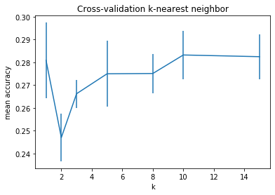
There is no immediate reason as to why an algorithm such as k-nearest-neighbors would even show any conclusive results on the raw input data. Things like camera perspective transformation, object displacement/rotation, color tints should make it very hard to classify images by comparing single pixel values. Yet, we come close to a 30% accuracy (compared to 10%, if the algorithm was plain random). The performance of knn depends on the representation of the data. If we had a better feature map, which could transform our data in to highly abstracted and meaningful features, then our algorithm would show a better performance. Conversely, when parsing a neural network’s decision, for example, often the maximum value of the class probabilities is chosen (which is 1-nearest-neighbor). If we were to remove the last layer and use the neural network’s feature representation combined with knn, we could see a performance boost (see Christopher Olah’s Blog for more details).