Dreaming of Tensors

In machine learning, the backpropagation algorithm requires us to calculate the gradient of a loss or cost functions $c:\R^{m\x n}\to \R$. In doing so, the chain rule is applied and derivatives of intermediate matrix functions $f:\R^{m\x n}\to \R^{m\x n}$ have to be evaluated. This article aims to showcase a practical approach in evaluating such expressions and to further an understanding of the derivative and its use in backpropagation.

The derivative in higher dimensions

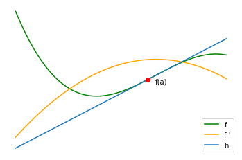
one dimension

In the above, 1-dimensional example, it is common use the words derivative and slope interchangeably.
For example, by calculating the affine linear approximation $h$ (also known as the first-order Taylor expansion of $f$ in point $a$), we may write

$h(x) = f(a) + f'(a)(x-a)$

or by substitution:

$h(a + t) = f(a) + f'(a)t\tag{1}$

and multiply our direction $t$ with the function’s slope at point $a$.

For a single input and a single output the rate of change of the function directly corresponds to the slope of the graph.

In the multivariable, scalarfield case, where a scalar output depends on multiple inputs, we require a direction in which to measure the slope of the graph.

In order to further extend the notion of a derivative to higher dimensions, the multiplication in $(1)$ could be seen as a linear function:

$h(a+t) = f(a) + l(t)$

where $l(t) = f'(a)t$ is a linear mapping from $\R$ to $\R$. Linear mappings from $\R$ to $\R$ are noted as $\L(\R,\R)$.
The derivative $f'$ then is a function $\R \to \L(\R,\R)$, which takes as input any arbitrary point $a$ and yields the linear approximation $l:\R \to \R$ of $f$ in point $a$.

scalar-by-vector

given a scalarfield, a function $f:\R^d \to \R$, the derivative at point $x$ is the best linear approximation $L:\R^d \to \R$ of $f$ in point $x$, denoted as $Df(x)$.

$Df(x)(v) = \sum_i\pd{f(x)}{x_i}v_i = (\nabla f(x))^\top v$
where

$\nabla f(x) = \pmatrix{\pd{f(x)}{x_1} \\ \vdots \\ \pd{f(x)}{x_d}}$

Reminder:

$\begin{aligned} Df:\R^d &\rightarrow \mathcal L (\R^d,\R) \\ x &\mapsto Df(x) \end{aligned}$

$\underset{\in \L(\R^d,\R)}{Df(x)} \neq \underset{\in \R^d}{\nabla f(x)}$

$Df(x)$ is actually not $\nabla f(x)$, since the former is a linear function $\in \L(\R^d,\R)$ (also called the dual of $\R^d$) while the latter is a vector, an element of $\R^d$. Because of the natural isomorphism $\L(\R^d,\R) \cong \R^d$ we may identify a linear map to $\R$ by a vector (by making use of the scalar-product). I will commit the occasional sin of mixing these notions, for example when writing $\nabla f(x) = Df(x)^\top$, but it should be pointed out that these are essentially two different types of objects.

As an interesting side note, ...

the Riesz representation theorem, a fundamental theorem in functional analysis (a generalization of this idea) states that for any Hilbert space $\H$ (a vector space which is complete by its scalar-product induced norm), each dual element $l \in \H^* = \L(\H, \R)$) (the space of linearly continuous functionals) is representable by an element $y_l \in \H$ of the space itself (even in the infinite dimensional setting). The application of the functional is equivalent to applying the scalar product to said element: $l(x) = _\H$. In the finite dimensional setting, every inner product space is complete and any linear function is continuous.

As before, via Taylor-Expansion, we can compute the first-order approximation of $f$ by

$f(x+tv) \approx f(x) + Df(x)(v)t$

Now you might be asking yourself whether to think of the derivative as a gradient or as a linear transformation. The idea of a gradient does not extend well to the multivariate case, i.e. a function $f:\R^d \to \R^d$ with multiple outputs, as it is not immediately an object of your input space anymore. The notion of a linear transformation however still holds. I will sometimes simply refer to derivatives as tensors, leaving the question of what type of object it is in the open.

vector-by-vector

In the multivariate case of $f:\R^d \to \R^n, \; f(x_1,..,x_d) = \begin{pmatrix}f_1(x_1,..,x_d) \\ \vdots \\ f_n(x_1,..,x_d)\end{pmatrix}$ we are looking for a function $Df$ that takes a vector as input, and returns a linear transformation $\mathcal L(\R^d, \R^n)$ which is representable by a matrix $\R^{n\times d}$ and the application of the transformation being the equivalent of performing a matrix multiplication. $Df \cong J_f$, the Jacobian of the function.

$J_f(x) = \jacobian{f(x)}{x}{n}{d} \in \R^{n\times d}$

$\forall x \in \R^d, v \in \R^d: Df(x)(v) = J_f(x)v$

In this case, $Df$ can be equivalently seen as a mapping $\R^d \to \R^{n\times d}, \; x \mapsto J_f(x)$

Some examples:

$\begin{aligned} f(x_1, x_2) &= \pmatrix{x_1+x_2 \\ x_2^2 \\ e^{x_1}} \\ J_f(x) &= \bmatrix{1 & 2 \\ 0 & 2x_2\\ e^{x_1} & 0} \\ J_f{(0,2)} &= \bmatrix{1 & 2 \\ 0 & 4 \\ 1 & 0} \end{aligned}$

This points out that $J_f$ first needs to be evaluated before obtaining the linear approximation.
Other examples include:

matrix multiplication:

$\begin{aligned} f(x) = Ax &= \pmatrix{a_{11}x_1 + .. + a_{1d}x_d \\ \vdots \\ a_{n1}x_1 + .. + a_{nd}x_d} \\ J_f(x) &= \matrixfill{a}{n}{d} = A \end{aligned}$

This function is constant and the matrix does not have to be evaluated (the derivative of a linear function is the same for all inputs $x$). And

$Df(x)(v) = Av$

activation functions:

$f(x) = \pmatrix{\sigma (x_1) \\ \vdots \\ \sigma (x_1)}, J_f(x) = \bmatrix{\sigma '(x_1) & 0 & \cdots & 0 \\ 0 & \sigma '(x_2) & & \vdots\\ \vdots& & \ddots & \\ 0 & \cdots & & \sigma '(x_d)}$

$Df(x)(h) = \pmatrix{\sigma '(x_1)h_1 \\ \vdots \\ \sigma '(x_d)h_d} = \pmatrix{\sigma '(x_1) \\ \vdots \\ \sigma '(x_d)} \odot \pmatrix{h_1 \\ \vdots \\ h_d}$

Thus, if an activation function is applied element-wise, the resulting derivative can also be computed element-wise. The application of the derivative can be written using the $\odot$ Hadamard (element-wise) Product.

With the the stage set for the basic derivatives we can have a look at the basic idea of the backpropagation algorithm.

The idea behind backpropagation

When modelling a neural network for example we always need a loss function which we can minimize. The loss function is essentially a function $f:\R^d \to \R$, it takes an input $x$ and returns a scalar, the loss.

Note, that in the case of a neural network we might be minimizing over the weights $W$, then $f$ is a function $\R^{h_2\x h_1} \to \R$, but this is practically the same as $\R^{h_2\cdot h_1} \to \R$. More on this later…

If $f$ is differentiable, a step of the backpropagation algorithm is performed by computing $x_{new}$ using the update rule $x_{new} = x - \lambda \nabla f(x)$.

By Taylor-Expansion, we know that:

$f(x+tv) = f(x) + Df(x)(v)t + o(t^2)$

where $o(t^2)$ is the error-term that decays quadratically in $t$ (this means that for very small $t$ this term will be of ‘lesser importance’ and the linear term will outweigh the quadratic $t^2$-term).
Evaluating for $x_{new}$ gives us:

$\begin{aligned} f(x_{new}) &= f(x-\lambda \nabla f(x)) \\&= f(x) + - \lambda (\nabla f(x))^\top \nabla f(x) + o(\lambda ^2) \\&= f(x) -\lambda \| \nabla f(x)\|^2 + o(\lambda ^2) \end{aligned}$

$\Rightarrow f(x_{new}) - f(x) = -\lambda \| \nabla f(x)\|^2 + o(\lambda ^2)$

This means that, since the squared norm $\|\nabla f(x)\|^2$ is positive, if we choose $\lambda$ small enough, then the right-hand side $-\lambda \| \nabla f(x)\|^2 + o(\lambda ^2)$ will be negative and thus

$\begin{aligned}f(x_{new}) - f(x) &\leq 0 \\ \Rightarrow f(x_{new}) &\leq f(x) \end{aligned}$

In neural networks one might have $g:\R^d\to \R^m$ as an intermediate function and $f:\R^m \to \R$ with our the cost being $c = f(g(x))$. Using the chain rule, we obtain:

$\begin{aligned} \nabla c(x) &= \nabla (f\circ g)(x) = J_{f\circ g}(x)^\top \\ &=\left (J_f({g(x)})J_g(x) \right)^\top = J_g(x)^\top J_f({g(x)})^\top \\ &= J_g(x)^\top \nabla f(g(x)) = J_g(x)^\top \nabla c(g(x))\end{aligned}$

$\begin{aligned} &\R^d& &\overset{g}\to& &\R^m& &\overset{f}\to& \R \\ &x& &\mapsto& &g& &\mapsto& c \\ &\nabla _x c& &\overset{J_g(x)^\top}{\leftmapsto}& &\nabla c(g)& \end{aligned}$

which illustrates how the gradient propagated from “front to back”. Note that, since the derivatives have to be evaluated at their respective positions this also explains why we would want to store intermediate variables such as $g$ in a cache as to not have to recompute these values every time.

scalar-by-matrix

One might think that a derivative of a scalar by a matrix would surely be a matrix as well, although following our definition of the derivative as a linear transformation, given $f:\R^{m\x n} \to \R$, we expect the derivative $Df(x)$ to be $\in \L(\R^{m\x n}, \R)$ a linear function that takes as input a matrix and outputs a scalar.

Yet, using standard notation there is no matrix that converts another matrix into a scalar, as applying a matrix ‘from the right’ will look like matrix multiplication. A way to get around this problem would be to vectorize our input, keeping the order of the elements:

$X \in \R^{m\x n}= \matrixfill{x}{m}{n} \cong \pmatrix{x_{11} \\ \vdots \\ x_{1n} \\ \vdots \\ x_{d1} \\ \vdots \\ x_{dn}} = \vec X \in \R^{m\cdot n}$

$f(X) = \tilde f(\vec{X})$

In this case, we are looking at a function $\tilde f:\R^{m\cdot n} \to \R$ which we already covered in the $\pd{scalar}{vec}$ case. The derivative then is
$Df(X) \cong \nabla \tilde f(\vec{X}) \in \R^{m\cdot n}$.

$D\tilde f \cong \pmatrix{\pd{f}{x_{11}} \cdots \pd{f}{x_{1n}} \cdots \pd{f}{x_{d1}} \cdots \pd{f}{x_{dn}}}$

Applying this derivative to a matrix $H$:

$Df(X)(H) = \nabla \tilde f(\vec{X}) \cdot (\vec{H}) = \sum_{ij} \pd{f(X)}{x_{ij}}h_{ij}$

where $\cdot$ is the vector scalar-product.
Or simply

$\pd{f(X)}{x_{ij}}h_{ij}$

using the Einstein summation convention where corresponding upper and lower indices are summed. For example

$\sum_{i}f_{i}e^{i} \quad \text{and} \quad \sum_{j}f_{ij}e^{jk}$

become

$f_{i}e^{i} \quad \text{and} \quad f_{ij}e^{jk}$

We might still decide that we want to write our derivative as a matrix. This is useful in the case that we want to calculate the ‘gradient’ for an update rule or when using the chain rule.

$\pd{f(X)}{X}^\top \cong \pdmatrix{f(X)}{x}{m}{n} \in \R^{m\x n}$

Thus far the matrix numerator-layout was used. Following this layout the derivative would have to be a $n\x m$ (transposed) matrix. To keep consistency in notation (which is important while applying the chain rule) I will refer to the gradient as $\pd f X ^\top$ which has the same dimensions as $X$ ($m\x n$).

In the following I will assume that all derivatives are written in their matrix/tensorial form evaluated at their respective inputs and I will refer to the gradient (the transposed tensorial form) as

$\pd{f(X)}{X}^\top \text{ or } \pd{f}{X}^\top \in \R^{m\x n}$

$\begin{aligned} Df(X)(H) &= \pd{f}{X}^\top \bullet H \\ &= \sum \left(\pdmatrix{f}{x}{m}{n} \odot \matrixfill{h}{m}{n}\right) \\ &= \sum \matrixeval{\pd{f}{x_{\i\j}}h_{\i\j}}{m}{n} \\ &= \pd{f}{x_{ij}}h_{ij} \\ \end{aligned}$

where “$\bullet$” means we calculate the element-wise product and then sum all entries. “$\bullet$” is basically the dot scalar-product if we were to vectorize matrices.

example of a scalar-matrix derivative:

An example is the (squared and rescaled) Frobenius matrix norm:

$f:\R^{m\x n}\to \R, \quad X \mapsto \frac{1}{2}\|X\|_F^2 = \frac{1}{2}\sum_{ij}x_{ij}^2$

$\pd{f(X)}{X}^\top \cong \matrixfill{x}{m}{n} = X$

$Df(\mathbb{1}_{m\x n})(Y) = \mathbb{1}_{m\x n} \bullet Y = \sum_{i,j} y_{ij}$

Here, I also want to note that depending on how we wish to contract a tensor

$\pd{f}{x_{ij}} \cong \R^{m\x n}$

this can be seen as an element $\in \L(\R^m,\R^n)$, which corresponds to normal matrix-multiplication:

$\pd{f}{x_{ij}}a_j \text{ where $a \in \R^m$}$

an element $\in \L(\R^n,\R^m)$ (transposed matrix-multiplication):

$b_i\pd{f}{x_{ij}} \text{ where $b \in \R^n$}$

or an element $\in \L(\R^{m\x n},\R)$, as we have seen:

$\pd{f}{x_{ij}}h_{ij} \text{ where $H \in \R^{m\x n}$}$

just by noting the indices along which we wish to contract a tensor. In this sense, the Einstein notation proves to be very elegant.

matrix-by-matrix

Assume we have a function $A:\R^{p\x q} \to \R^{m\x n}$ and $c:\R^{m\x n} \to \R$ (this could be an activation layer and a cost function in a neural network).

$\begin{aligned} &\R^{p\x q}& &\to& &\R^{m\x n}& &\to& \R \\ &X& &\mapsto& &A& &\mapsto& c \\ \end{aligned}$

Applying the chain rule:

$\pd{c}{x_{kl}} = \pd{c}{a_{ij}}\pd{a_{ij}}{x_{kl}}$

We eventually come across the term

$\pd{a_{ij}}{x_{kl}}$

which, as the 4 indices indicate, is a rank-4 tensor.

Since we are interested in the gradient, we wish to calculate (again, sorry for the abuse of notation)

$\pd{c}{X}^\top \in \R^{p\x q}, \quad \pd{c}{X}^\top = \left(\pd{c}{A}\pd{A}{X}\right)^\top = \pd{A}{X}^\top\pd{c}{A}^\top$

where

$\pd{c}{A}^\top = \pdmatrix{c}{a}{m}{n} \in \R^{m\x n}$

$\pd{A}{X}^\top = \pdmatrix{A}{x}{p}{q} \in \R^{(p\x q)\x(m\x n)}$

And $\R^{(p\x q)\x(m\x n)}$ is seen as a linear transformation $\L(\R^{m\x n},\R^{p\x q})$

The single entries of the gradient are

$\pd{c}{x_{kl}} = \pd{a_{ij}}{x_{kl}}\pd{c}{a_{ij}}$

Note: this formula encapsules everything one needs to know on how to calculate a derivative. However, keeping track of all those indices can get confusing. The way one could proceed to evaluate such an expression while keeping the spatial structure of the matrix is as follows.

Using the recently introduced notation:

$\pd{A}{x_{kl}} \bullet \pd{c}{A}^\top = \sum \pd{A}{x_{kl}} \odot \pd{c}{A}^\top$

, where we sum over all free indices.
This means we can expand the tensor along the $p\x q$ dimensions and contract the other dimensions using the Hadamard product and summing. In almost the same fashion that we can calculate each entry of a matrix product by overlaying column and row vectors and then summing, here we overlay the matrix $\pd{c}{A}^\top$ with each $\pd{A}{x_{kl}}$ (also a matrix) and then sum.

In total, we then obtain:

$\pd{c}{X}^\top = \pd{A}{X}^\top \pd{c}{A}^\top = \matrixeval{\pd{a_{ij}}{x_{\i\j}} \pd{c}{a_{ij}}}{p}{q}$

$= \matrixplace{ \color{darkviolet}{\pd{A}{x_{11}}} \color{black}{\bullet}\color{dodgerblue}{\pd{c}{A}^\top} }{ \pd{A}{x_{1q}} \bullet \color{dodgerblue}{\pd{c}{A}^\top} }{ \pd{A}{x_{p1}} \bullet \color{dodgerblue}{\pd{c}{A}^\top} }{ \pd{A}{x_{pq}} \bullet \color{dodgerblue}{\pd{c}{A}^\top} }$

$= \matrixplace{ \sum\matrixeval{ \color{darkviolet}{ \pd{a_{\i\j}}{x_{11}} } \color{dodgerblue}{ \pd{c}{a_{\i\j}} } }{m}{n} }{ \sum\matrixeval{ \pd{a_{\i\j}}{x_{1q}} \color{dodgerblue}{ \pd{c}{a_{\i\j}} } }{m}{n} }{ \sum\matrixeval{ \pd{a_{\i\j}}{x_{p1}} \color{dodgerblue}{ \pd{c}{a_{\i\j}} } }{m}{n} }{ \sum\matrixeval{ \pd{a_{\i\j}}{x_{pq}} \color{dodgerblue}{ \pd{c}{a_{\i\j}} } }{m}{n} }$

An example might clear things up.

---

Given an affine linear function

$Z(W) = WX + b$

where $X \in \R^{q\x n}$

$\begin{aligned} &\R^{p\x q}& &\to& &\R^{p\x n}& \\ &W& &\mapsto& &Z& \\ \end{aligned}$

The gradient can be written as

$\pd{Z}{W}^\top = \pdmatrix{Z}{w}{m}{n} \in \R^{(p\x q)\x(p\x n)}$

, as a linear transformation $\L(\R^{p\x n},\R^{p\x q})$.

The constant part $b$ is not relevant when calculating the derivative and can be ignored.

$\begin{aligned} WX &= \matrixfill{w}{p}{q} \matrixfill{x}{r}{n} \\ &= \matrixeval{\sum_k w_{\i k}x_{k\j}}{m}{n} \end{aligned}$

Evaluating $\pd{Z}{w_{ij}}$ gives

$\begin{matrix} \pd{Z}{w_{11}} = \bmatrix{ x_{11} & x_{12} & \cdots & x_{1n} \\ 0 & 0 & & 0 \\ \vdots & & \ddots & 0 \\ 0 & 0 & 0 & 0 \\ } & \pd{Z}{w_{12}} = \bmatrix{ x_{21} & x_{22} & \cdots & x_{2n} \\ 0 & 0 & & 0 \\ \vdots & & \ddots & 0 \\ 0 & 0 & 0 & 0 \\ } & \cdots \\ \\ \pd{Z}{w_{21}} = \bmatrix{ 0 & 0 & & 0 \\ x_{11} & x_{12} & \cdots & x_{1n} \\ \vdots & & \ddots & 0 \\ 0 & 0 & 0 & 0 \\ } & \pd{Z}{w_{22}} = \bmatrix{ 0 & 0 & & 0 \\ x_{21} & x_{22} & \cdots & x_{2n} \\ \vdots & & \ddots & 0 \\ 0 & 0 & 0 & 0 \\ } \\ \vdots \end{matrix}$

Recalling how to apply the derivative $\pdt Z W$ to a matrix $H$ (when training neuronal nets, this is typically $dZ$), we multiply each of the above submatrices with $H$ element-wise and then sum all entries.

$\pdt Z W (H) = \matrixeval{\sum h_{\i k}x_{\j k}}{m}{n} = HX^\top$

The next example was the motivation for writing this article.

cross-entropy loss & softmax

given functions $A:\R^{m\x n} \to \R^{m\x n}$ and $c:\R^{m\x n} \to \R$

$\begin{aligned} &\R^{m\x n}& &\to& &\R^{m\x n}& &\to& \R \\ &X& &\mapsto& &A& &\mapsto& c \\ \end{aligned}$

where $c$ is the cross-entropy loss:

$c(A) = -\frac{1}{n}\sum_{ij}y_{ij}ln(a_{ij})$

and $A$ is the softmax-activation:

$A(X) = \matrixeval{\frac{e^{x_{\i\j}}}{\sum_ze^{x_{z\j}}}}{m}{n}$

where the column vectors are normalized by the sum of each column, so that they add to 1.

Using our chain rule for the gradient:

$\pd{c}{X}^\top = \pd{A}{X}^\top \pd{c}{A}^\top$

$\begin{aligned} \pd{c}{A}^\top &=&\matrixeval{\pd{c}{a_{\i\j}}}{m}{n}& \\ &=& -\frac{1}{n} \matrixeval{ \frac{y_{\i\j}}{a_{\i\j}} }{m}{n}& =-\frac{1}{n} Y \oslash A \end{aligned}$

as $\odot$ is the operator for element-wise multiplication, $\oslash$ will denote element-wise division.

$\pd{A}{X}^\top = \pdmatrix{A}{x}{p}{q} \in \R^{(p\x q)\x(m\x n)}$

as evaluating

$\pd{}{x_{kl}} \left( \frac{e^{x_{ij}}}{\sum_ze^{x_{zj}}} \right) = 0 \quad \text{ if l $\neq$ j}$

becomes a headache with all those indices, I will go through the first few examples. The pattern will then become clear.

$\begin{aligned} \pd{a_{11}}{x_{11}} &= \pd{}{x_{11}} \left( \frac{e^{x_{11}}}{\sum_ze^{x_{z1}}} \right) \\ &= \frac{e^{x_{11}}}{\sum_ze^{x_{z1}}} - e^{x_{11}} \frac{1}{\left( \sum_ze^{x_{z1}} \right)^2}e^{x_{11}} \\ &= \frac{e^{x_{11}}}{\sum_ze^{x_{z1}}}\left(1 - \frac{e^{x_{11}}}{\sum_ze^{x_{z1}}}\right) \\ &= a_{11}(1-a_{11}) \\ \pd{a_{21}}{x_{11}} &= \pd{}{x_{11}} \left( \frac{e^{x_{21}}}{\sum_ze^{x_{z1}}} \right) \\ &= 0 - e^{x_{21}} \frac{1}{\left( \sum_ze^{x_{z1}} \right)^2}e^{x_{11}} \\ &= -a_{11}a_{21} \\ \pd{a_{31}}{x_{11}} &= -a_{11}a_{31} \\ &\vdots \end{aligned}$

and if the columns are not aligned:

$\pd{a_{12}}{x_{11}} = 0$

In full, we have:

$\begin{aligned} \pd{A}{x_{11}} &= \bmatrix{ -a_{11}(a_{11}-1) & 0 & & 0 \\ -a_{11}a_{21} & 0 & \cdots & 0 \\ -a_{11}a_{31} & 0 & & 0 \\ \vdots & & \ddots & \vdots \\ -a_{11}a_{m1} & 0 & \cdots & 0 \\ } \\ &= -A \odot \bmatrix{ (a_{11}-1) & 0 & & 0 \\ a_{11} & 0 & \cdots & 0 \\ a_{11} & 0 & & 0 \\ \vdots & & \ddots & \vdots \\ a_{11} & 0 & \cdots & 0 \\ } \end{aligned}$

for all entries:

$\begin{matrix} \pd{A}{x_{11}} = -A \odot \bmatrix{ (a_{11}-1) & 0 & & 0 \\ a_{11} & 0 & \cdots & 0 \\ a_{11} & 0 & & 0 \\ \vdots & & \ddots & \vdots \\ a_{11} & 0 & \cdots & 0 \\ } & \pd{A}{x_{12}} = -A \odot \bmatrix{ 0 & (a_{12}-1) & 0 & & 0 \\ 0 & a_{12} & 0 & \cdots & 0 \\ 0 & a_{12} & 0 & & 0 \\ & \vdots & & \ddots & \vdots \\ 0 & a_{12} & 0 & \cdots & 0 \\ } & \cdots \\ & \\ \pd{A}{x_{21}} = -A \odot \bmatrix{ a_{21} & 0 & & 0 \\ (a_{21}-1) & 0 & \cdots & 0 \\ a_{21} & 0 & & 0 \\ \vdots & & \ddots & \vdots \\ a_{21} & 0 & \cdots & 0 \\ } & \pd{A}{x_{22}} = -A \odot \bmatrix{ 0 & a_{22} & 0 & & 0 \\ 0 & (a_{22}-1) & 0 & \cdots & 0 \\ 0 & a_{22} & 0 & & 0 \\ & \vdots & & \ddots & \vdots \\ 0 & a_{22} & 0 & \cdots & 0 \\ } & \cdots \\ \vdots \end{matrix}$

Now, when contracting each of these matrices with $\pd{c}{A}^\top = -\frac{1}{n}Y\oslash A$:

For each entry, we ‘overlay’ the matrices and sum (overlaying means applying the element-wise product).

$\begin{aligned} \left[\pd{c}{X}\right]^\top_{11} &= \sum -A \odot \bmatrix{ (a_{11}-1) & 0 & & 0 \\ a_{11} & 0 & \cdots & 0 \\ a_{11} & 0 & & 0 \\ \vdots & & \ddots & \vdots \\ a_{11} & 0 & \cdots & 0 \\ } \odot -\frac{1}{n}Y\oslash A \\ &= \frac{1}{n} \sum \bmatrix{ y_{11}(a_{11}-1) & 0 & & 0 \\ y_{21}a_{11} & 0 & \cdots & 0 \\ y_{31}a_{11} & 0 & & 0 \\ \vdots & & \ddots & \vdots \\ y_{m1}a_{11} & 0 & \cdots & 0 \\ } \\ &= \frac{1}{n}(a_{11}\left(\sum_i y_{i1}\right) - y_{11}) \end{aligned}$

As all operations are element-wise, we can rearrange the operations, just like with normal multiplication.

if Y is a probability distribution, then the columns will each sum to one: $\sum_i y_{i1} = 1$. And we obtain $\pd{c}{x_{11}} = \frac{1}{n}(a_{11} - y_{11})$

In total we have:

$\pd{c}{X}^\top = \bmatrix{ \frac{1}{n}(a_{11} - y_{11}) &\frac{1}{n}(a_{12} - y_{12}) & \cdots \\ & \\ \frac{1}{n}(a_{21} - y_{21}) &\frac{1}{n}(a_{22} - y_{22}) \\ & \\ \vdots & & \ddots }$

Thus the gradient is simplified to:

$\pd{c}{X}^\top = \frac{1}{n}( A - Y)$