The focus of this article will be on the math behind simple neural networks and implementing the code in python from scratch. Also, the differences between binary and multiclass models will be highlighted.
This article tries to be as detailed as necessary in covering each derivation of the formulas, so that every line of code can be comprehended. This might not be a guide for complete beginners, as some basic knowledge in linear algebra is required.
primer

A neural network, simply put, a function that maps input to output. The dimensions of the input/output and its inner topology all are variable. The function itself is not explicitly defined beforehand, but inferred from the dataset.
Example of a neural network mapping input to output .
The inputs and outputs will be column vectors, as I find that more intuitive when working with matrices. This is an arbitrary convention and can is easily changed by transposition.
We can also run a batch of samples through the neural network.
Different datapoints will be noted as upper indices in parentheses, the individual entries as lower indices.
The propagation from one layer to the next consists of an affine linear transformation, , followed by a non-linear activation function , applied element-wise.
is a matrix (here, a linear Transformation from to ) and the bias is a scalar .
A neural network may be composed of multiple layers. Each layer acting on the previous layer’s output or “neural activation”.
Upper indices in brackets denote the layer from to .
It would seem more logical to start with the general multiclass model and then to study the binary model as a special case. Nonetheless, I will begin with the binary model, since calculating derivatives and predicting is simpler in this case.
binary classification

The regular multiclass model assumes two output dimensions, each representing the probability of the sample belonging to the respective class or . Yet, as the probability of belonging to 'class ’ is minus the probability of belonging to 'class ': , and vice-versa, one output variable becomes redundant. Only one output ‘neuron’ is needed.
The estimated probability of whether the input belongs to each class, given our model then is
, where .
imports
Numpy will be used for matrix calculations and matplotlib for plots. Later, scikit will help in creating a toy dataset.
import numpy as np | |
import matplotlib.pyplot as plt | |
import sklearn.datasets | |
initialization
The function nn_init() initializes a neural network with random weights and zero bias. It takes a parameter layer_dims, an array specifying the number of neurons for each layer. layer_dims = [2, 8, 1] for example. The first entry is the input dimension and reflects the dimension of the data, the last is the network’s output dimension and is equal to the number of classes in the general case.
The function returns a dictionary param containing the network’s information.
The weights connecting the input to the first layer are stored in param['W1'], the bias in param['b1'], and so on. The number of layers is len(layer_dims) - 1 (not counting the input layer).
def nn_init(layer_dims): | |
L = len(layer_dims) - 1 | |
param = {'L': L} | |
for l in range(1, L + 1): | |
param['W' + str(l)] = np.random.randn(layer_dims[l], layer_dims[l-1]) | |
param['b' + str(l)] = np.zeros((layer_dims[l], 1)) | |
return param | |
forward pass
A nonlinear activation function is applied to each layer after the affine linear transformation. The hidden layers will all be equipped with the rectified linear unit, or relu-activation function.
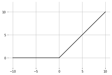
def relu(Z): | |
return Z * (Z > 0) | |
The last layer will use the activation function. This way, the final output will be squished to values between and which then can be used for predicting the classes.
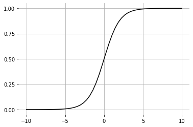
def sigmoid(Z): | |
return 1 / (1 + np.exp(-Z)) | |
Each layer’s activation is calculated as follows:
The forward pass begins with the input (a single sample or a batch) and iterates over the layers.
def nn_forward(X, param): | |
L = param['L'] | |
A = X | |
cache = {'A0': A } | |
for l in range(1, L + 1): | |
W = param['W' + str(l)] | |
b = param['b' + str(l)] | |
Z = W @ A + b | |
A = relu(Z) if l != L else sigmoid(Z) | |
cache['A' + str(l)] = A | |
return A, cache | |
All activations () are stored in the dictionary named cache, and the input in cache['A0'].
loss function
For our network to be able to learn anything, we need to formulate a loss function. For classification tasks, the cross-entropy loss function is a common choice. Its formulation for one sample is:
, where the sum is over all possible classes .
is the true probability of the sample belonging to class , and
is the predicted probability given the neural network model .
For the binary case, where the class labels are either or , the sum expands to
The true probability of a sample belonging to ‘class 1’ is reflected by its label.
And the true probability of not belonging to ‘class 1’, but ‘class 0’ is
Similarly, are the network’s predictions, the last layer’s output .
The binary loss function then is simplified to:
For a batch of samples , the loss can be averaged.
As a reminder:
For now, and are row-vectors, and and scalars, since the output has only one dimension. Later, in the multivariate case, these will be matrices and vectors respectively.
In python:
def loss(A, Y): | |
N = A.shape[1] | |
return np.sum(Y * np.log(A) + (1 - Y) * np.log(1 - A)) / -N | |
backward pass
Gradient descent is like a blind man trying to reach the bottom of a hill. He is only able to feel the hill’s slope with his feet and take small steps in the hill’s downward direction.
A derivative of a function similarly reflects the rate of change (or slope when graphed) of a parameter. It essentially says how much the output will change by a small tweak in input. In the multivariable case, the gradient points towards the direction of biggest (positive) change in output. In order to drive the network to a lower loss, all parameters are moved in the opposite direction of their gradients, in the ‘direction of negative slope’, by a small amount. Although, in general, this does not guarantee a reduce in cost.
The network’s parameters are its weights and biases. Thus, the gradients and need to be evaluated for each layer. For this, the derivatives of the activation functions, the loss and the affine linear functions need to be calculated.
In the case of (the loss function), where (a scalar) is dependent on (a matrix), which, in turn is dependent on (a matrix), evaluating the derivative w.r.t. can be done for all indices using the following chain rule:
In matrix form this is often written as
A word of warning. It is easy to make mistakes using the matrix version of the chain rule without knowing what is going on under the hood. Note that for example, is a 4-tensor and the derivative is a linear transformation from to , which cannot even be represented as a matrix using conventional notation. Even if we, nonetheless, decide to write the derivative as a matrix, keeping consistency with the numerator layout would make it a matrix of size . That is why I choose to write when referring to the gradient which has the same dimensions as . I further clarify this .
Rewriting the above equation yields
or
And it can be seen how, in order to calculate the desired derivative , the gradient is ‘backpropagated’.
cross-entropy loss
The cross-entropy loss function
has the following gradient:
Where the expression above is meant to be performed element-wise.
This can be seen by calculating the derivative w.r.t. one sample. Then and become scalars:
As the summands are independent of each other, the gradient can be written in the above, vectorized form.
activation functions
relu:
sigmoid:
Where the chain-rule was applied in the first equation.
affine linear functions
Given an affine linear function , the derivatives are and .
A derivation can be found . Many matrix derivatives can also be looked up in the matrix cookbook.
piecing together
Before implementing the code in python, I believe it is helpful to run through a small 2-layer example, from which the general algorithm can be derived. The aim is to evaluate and for each layer.
‘*’ and ‘/’ on matrices are used to indicate element-wise actions, keeping close to python’s syntax.
Making sure that the gradients match the dimensions of the variables also can prove helpful. For example one should be able to verify that A2.shape == dA2.shape.
The backpropagation through the last layer can be further simplified, as it is only necessary to calculate .
This step also prevents numerical errors that could arise when is close to or .
Implementation:
def relu_backward(Z): | |
return Z > 0 | |
def last_layer_backward(A, Y): | |
N = A.shape[1] | |
return (A * (1-Y) - Y * (1-A)) / N | |
def nn_backward(Y, param, cache): | |
L = param['L'] | |
A = cache['A' + str(L)] | |
N = A.shape[1] | |
grad = {} | |
for l in reversed(range(1, L + 1)): | |
A_prev = cache['A' + str(l-1)] | |
W = param['W' + str(l)] | |
dZ = dA * relu_backward(A) if l !=L else last_layer_backward(A, Y) | |
grad['dW' + str(l)] = dZ @ A_prev.T | |
grad['db' + str(l)] = dZ.sum(axis=1, keepdims=True) | |
dA = W.T @ dZ | |
A = A_prev | |
return grad | |
parameter update
The parameters are updated using the following rule:
, given the learning rate .
def update_param(param, grad, learning_rate=0.01): | |
for l in range(1, param['L'] + 1): | |
param['W' + str(l)] -= grad['dW' + str(l)] * learning_rate | |
param['b' + str(l)] -= grad['db' + str(l)] * learning_rate | |
training
Training the neural network is achieved by iterating over the following steps:
- forward pass (evaluating for each layer)
- backward pass (computing the gradients and )
- parameter update (tuning the weights and biases)
A list of the computed costs can be stored for logging/graphing the network’s progress.
def train(X, Y, param, epochs=50000, learning_rate=0.001, | |
print_every=10000): | |
costs = [] | |
for epoch in range(epochs + 1): | |
A, cache = nn_forward(X, param) #1 | |
grad = nn_backward(Y, param, cache) #2 | |
update_param(param, grad, learning_rate) #3 | |
if epoch % print_every == 0: | |
cost = loss(A, Y) | |
costs.append(cost) | |
print('epoch {}, loss: {}'.format(epoch, cost)) | |
return costs | |
predicting and evaluation
When making a class prediction, the class with the higher probability is chosen. Thus, if the estimated probability for ‘class 1’ is greater than 0.5, the prediction is set to ‘class 1’, otherwise it will be ‘class 0’.
The networks empirical correct classification rate is
def predict(X, param): | |
A, _ = nn_forward(X, param) | |
return A > 0.5 | |
def evaluate_classifier(X, Y_true, param): | |
Y_pred = predict(X, param) | |
return np.mean(Y_pred == Y_true) | |
toy data
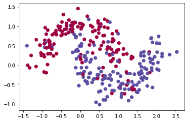
Sci-kit sklearn has built in functions to easily create datasets.
def load_dataset(): | |
n_samples = 300 | |
np.random.seed(0) | |
X, Y = sklearn.datasets.make_moons(n_samples=n_samples, noise=.2) | |
X = X.T | |
flip = np.random.choice(range(n_samples), 40) #add in some outliers | |
Y[flip] = 1 - Y[flip] | |
return X, Y | |
X, Y = load_dataset() | |
plt.scatter(X[0], X[1], c=Y, s=40, cmap='Spectral') | |
plt.show() | |
The dataset is shuffled and then split into two parts, a training and a testing dataset. The test set is used for evaluating the network’s ability to extrapolate on data it has never seen before.
def split_dataset(X, Y, ratio=0.8): | |
N = X.shape[1] | |
split = int(N * ratio) | |
shuffle = np.random.permutation(N) | |
X_train = X[:,shuffle[:split]] | |
X_test = X[:,shuffle[split:]] | |
Y_train = Y[shuffle[:split]] | |
Y_test = Y[shuffle[split:]] | |
return (X_train, Y_train), (X_test, Y_test) | |
(X_train, Y_train), (X_test, Y_test) = split_dataset(X, Y) | |
print('X_train shape: {}'.format(X_train.shape)) | |
print('Y_train shape: {}'.format(Y_train.shape)) | |
print('X_test shape: {}'.format(X_test.shape)) | |
print('Y_test shape: {}'.format(Y_test.shape)) | |
X_train shape: (2, 240)
Y_train shape: (240,)
X_test shape: (2, 60)
Y_test shape: (60,)
binary model
Now that all necessary building components are finished, it is time to assemble the network. The number of input dimensions can be read directly from the dataset (in this case the data is 2-dimensional) and the output uses one neuron in the binary case. The dimension of the hidden layer is somewhat arbitrarily set to 8. Passing the specified layer dimensions to the nn_init() function, the parameters of a randomly initialized neural network are returned. The network is then trained on the training dataset.
d_in = X_train.shape[0] | |
d_out = 1 | |
layer_dims = [d_in, 8, d_out] | |
param = nn_init(layer_dims) | |
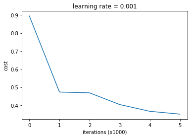
costs = train(X_train, Y_train, param, | |
epochs=500000, learning_rate=0.001, print_every=100000) | |
epoch 0, loss: 0.8943569024225951
epoch 100000, loss: 0.47308653964775604
epoch 200000, loss: 0.46855221922894785
epoch 300000, loss: 0.40372674060427743
epoch 400000, loss: 0.36625403094480086
epoch 500000, loss: 0.35062643425360634
The next part is about visualizing the performance of our network. It is not essential for understanding neural networks. The code of plot_decision_boundary is mostly adapted from scikit.
code for plot_costs, plot_decision_boundary
def plot_costs(costs, plot_every=1000, learning_rate=.001): | |
plt.plot(costs) | |
plt.ylabel('cost') | |
plt.xlabel('iterations (x{})'.format(plot_every)) | |
plt.title("learning rate = {}".format(learning_rate)) | |
plt.show() | |
def plot_decision_boundary(X, Y, param, contourgrad = False): | |
cmap = 'Spectral' | |
h = 0.01 | |
x_min, x_max = X[0,:].min() - 10*h, X[0,:].max() + 10*h | |
y_min, y_max = X[1,:].min() - 10*h, X[1,:].max() + 10*h | |
xx, yy = np.meshgrid(np.arange(x_min, x_max, h), | |
np.arange(y_min, y_max, h)) | |
mesh = (np.c_[xx.ravel(), yy.ravel()]).T | |
Z = predict(mesh, param) | |
Z = Z.T.reshape(xx.shape) | |
plt.figure(figsize=(5,5)) | |
if contourgrad: | |
A, _ = nn_forward(mesh, param) | |
plt.contourf(xx, yy, A.T.reshape(xx.shape), cmap=cmap, alpha=.3) | |
else: | |
plt.contourf(xx, yy, Z, cmap=cmap, alpha=.3) | |
plt.contour(xx, yy, Z, colors='k', linewidths=0.5) | |
plt.scatter(X[0,:], X[1,:], c=Y.squeeze(), cmap=cmap) | |
plt.show() | |
plot_costs(costs) | |
plot_decision_boundary(X_train, Y_train, param, contourgrad = True) | |
accuracy = evaluate_classifier(X_train, Y_train, param) | |
print('accuracy on train set: {}'.format(accuracy)) | |
accuracy = evaluate_classifier(X_test, Y_test, param) | |
print('accuracy on test set: {}'.format(accuracy)) | |
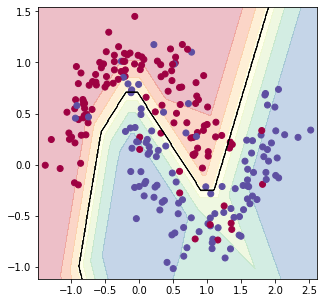
accuracy on train set: 0.8666666666666667
accuracy on test set: 0.8
multiclass neural network
The current network architecture only has one output neuron. Given, say, 10 classes, the network’s i-th output neuron then is to reflect the probability of the input belonging to ‘class i’.
As an example
Changing the current code-framework to be able to handle multiple classes involves the following:
- implementing the softmax layer, to be used as the last layer’s activation function
- revisiting the original cross-entropy loss formulation
- calculating the backward pass for the new last layer
- modifying the prediction function
softmax layer
After propagating the the input through an affine linear layer , can take on all sorts of values, positive or negative. If the 10 outputs are to reflect a probability distribution (i.e. have values between 0 and 1 that all sum to 1), the following can be done.
Each value is mapped to the exponential function, to ensure that it will be positive, and then divided by the sum of all outputs. The result can then be seen as a probability distribution.
This is exactly what softmax does:
As a side note: in the binary case it was redundant to work with two outputs, since the probability of not belonging to ‘class 1’ is simply
In that case
which can be substituted as
Again, we see the binary case emerge as a special case of the general case.
A numerical trick that is often employed in order to prevent the exponential term from blowing up (which may result in unstable computations) is the following:
is set to , the biggest value, to ensure numerical stability.
def softmax(Z): | |
A = np.exp(Z - np.max(Z, axis=0)) | |
return A / A.sum(axis=0) | |
cross-entropy loss
As a reminder, the loss for one sample is
, where is the one hot encoding of y.
The ‘one hat’ above the is supposed to remind of the one hot encoding.
Before, a scalar was used as a label for sample . = 3, as an example.
Now, with one hot encoding, it is assumed that is a vector of, say, length 10, with a ‘1’ at the index corresponding to the sample’s class, and ‘0’ everywhere else.
of ‘class 3’:
The class label data shape is the same as the neural network’s output.
To reduce overhead we can avoid explicitly converting our labels to one hot encodings by using numpy’s indexing.
Using numpy’s notation to access elements in arrays this would look like -log(a[y]).
For a batch of samples:
Using numpy’s advanced indexing, accessing these elements is done via A[Y, range(N)]. This expands to A[[Y(1), Y(2), ..], [1, 2, ..]], which then can be summed with np.sum.
def loss(A, Y): | |
N = A.shape[1] | |
return np.sum(np.log(A[Y, range(N)])) / -N | |
In deriving the theory, it is useful to stick to the one-hot formulation:
where the sum is over all free indices and ‘’ is the element-wise multiplication
From now on, to make it clearer, ‘’ and ‘’ will be used for element-wise multiplication and division.
backward pass
The goal is to calculate , the derivative of the last layer.
cross-entropy loss
The derivative of the cross-entropy loss
remains as before
, since all operations are still performed element-wise.
softmax layer
The derivative of the softmax layer is a bit more involved. The derivative of a matrix-function w.r.t. another matrix is a rank-4 tensor. I cover its full derivation via the chain rule .
Yet, we really only are interested in calculating (a matrix). And since the sum in the loss function involves independent terms and the softmax function acts on each sample individually, it is possible to calculate the derivative w.r.t. one input and then piece together the full derivative . The full derivative then becomes . And now, the term is a (more manageable) matrix.
With respect to one sample, the derivative of the loss function is
And the derivative of the softmax layer
is calculated as follows:
The product rule is used in after the first equation.
In full:
Combining both derivatives to obtain gives:
This is easier seen when expanding the matrices.
results in subtracting from the element of with the index corresponding to its true class.
The full derivative now is
In python, again, using advanced indexing:
def last_layer_backward(A, Y): | |
N = A.shape[1] | |
dZ = np.copy(A) #copy to not modify original | |
dZ[Y, range(N)] -= 1 | |
return dZ / N | |
predicting
The output layer contains the predicted class probabilities.
The final prediction is done by selecting the class with the highest estimated probability. This corresponds to the index of the highest value.
For a batch of samples this is done for each sample, i.e. each column of the matrix (axis 0 in numpy).
def predict(X, param): | |
A, _ = nn_forward(X, param) | |
return np.argmax(A, axis=0) | |
toy data
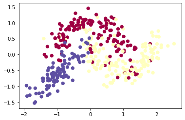
A toy dataset can be created by reusing the toy dataset for the binary case and adding multivariate normal distributed samples as a third class.
def load_dataset_multi(): | |
X, Y = load_dataset() | |
Z = np.random.multivariate_normal( [-5, -3], [[5, 4], [4, 5]], size=100) / 5 | |
X = np.concatenate((X, Z.T), axis=1) | |
Y = np.append(Y, (np.ones((1,100)) * 2).astype('int')) | |
plt.scatter(X[0], X[1], c=Y, s=40, cmap='Spectral'); | |
plt.show() | |
return X, Y | |
X, Y = load_dataset_multi() | |
(X_train, Y_train), (X_test, Y_test) = split_dataset(X, Y) | |
multiclass model
Finally, the multiclass neural network is initialized by specifying the layer dimensions and then is trained on the dataset, just as in the binary case.
d_in = X_train.shape[0] | |
d_out = Y_train.shape[0] | |
layer_dims = [d_in, 8, d_out] | |
param = nn_init(layer_dims) | |
train(X_train, Y_train, param, learning_rate=.001) | |
plot_decision_boundary(X_train, Y_train, param) | |
accuracy = evaluate_classifier(X_train, Y_train, param) | |
print('accuracy on train set: {}'.format(accuracy)) | |
accuracy = evaluate_classifier(X_test, Y_test, param) | |
print('accuracy on test set: {}'.format(accuracy)) | |
epoch 0, loss: 0.8492644177201928
epoch 10000, loss: 0.584044408860389
epoch 20000, loss: 0.5478712675155261
epoch 30000, loss: 0.5135834238863085
epoch 40000, loss: 0.500427787036695
epoch 50000, loss: 0.4898009397411907
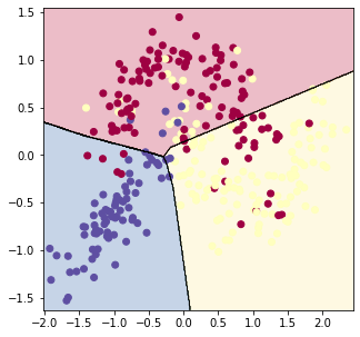
accuracy on train set: 0.8125
accuracy on test set: 0.75
The full python code can be found on my Github. Alternatively, the code can be run directly in a Google Colab notebook here.